LEFT, MID, & RIGHT

Have you ever had the need for data that's in a cell, but not the entire cell? When the need arises to dissect a cell, Excel has you covered.

Whether the data you need is in the beginning of a cell, the middle of a cell, or the end of a cell - there's a formula for that.

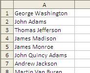
Where I work, we use a lot of dates in the format of YYYYMMDD (today is 20110430). Let's say you want to separate those into separate cells so you can subtotal them by their particular month. You need to figure out a way to split the cell so you can have the data you need. Because all of the data in this example is 8 characters long, there are a couple of different ways you can accomplish this; but today we're going to focus on using the LEFT, MID, & RIGHT formulas. Let's get right to it.

LEFT

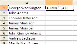
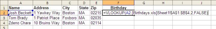
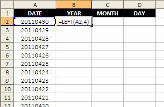
In order to extract the year from from the data, you use the LEFT formula. Before using this formula, you need to know two things; the cell that contains the data and the length of the data you'd like to extract. The formula takes the form of =LEFT(Cell that contains the data, the number of characters you'd like to extract). Here's a visual example:

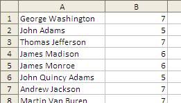
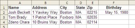
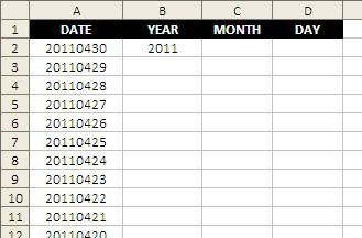
And the result:

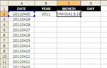
MID

To extract the month it's a little trickier (because it's in the MIDdle of the data), but it's still just as easy. This time you need to know THREE things before you can use the formula; the cell that contains the data, the position of the first character you want to extract, and the length of the data you'd like to extract. The formula takes the form of =MID(Cell that contains the data, the position of the first character you want to extract, the number of characters you'd like to extract). Here's a visual example:

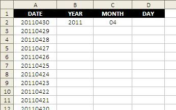
And the result:

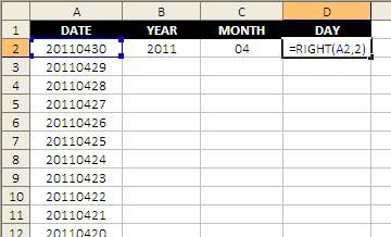
RIGHT

Using the RIGHT formula is just like using the LEFT formula except you're starting from the right instead of the left (it it weren't obvious enough!) Therefore, you need to know the same two things; the cell that contains the data and the length of the data you'd like to extract. The formula takes the form of =RIGHT(Cell that contains the data, the number of characters you'd like to extract). Here's a visual example:

And the result:

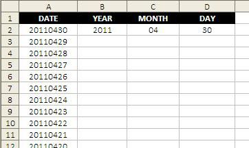
Here is the final result:

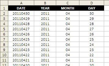
I hope I've explained it easy enough! At a later date, I'll explain the other method we could have used to accomplish this task - Text to Columns. As I stated earlier, only because every cell has the same amount of characters AND they are all in the same position (the first four positions are the year, the next two are the month, and the last two are the day) could we use this different method.


Until next time... Keep Excelling!!!

The FIND Function

If you need to know in which position a particular character is in a cell, the FIND function is exactly what you need.


Let's say you have a list of names. Both first and last name in one cell separated by a space. If by chance you want to know in which position the space is in, the formula is as simple as =FIND("What you're looking for", The cell that contains what you're looking for). That's it!


Here's a visual example.

Just remember that if what you're looking for is text, you need to enclose the search item in quotes (to find a space, we use " ")

As you can see the result is 7, meaning the space is the 7th character within that cell.

One other thing to keep in mind is that the formula will only find the first instance of what it is looking for. As you see in the example above on row 6, "John Quincy Adams" has 2 spaces, however the result of the formula is 5, meaning the space is in the 5th position. Once ANY formula finds what it is looking for, it stops looking and thus there is no mention of the 2nd space. (There is a way to find the 2nd and subsequent spaces, that's a little more advanced so it will be another topic for a later date).
 

Working with Multiple Tabs

Do you ever work with an Excel workbook that has multiple worksheets (tabs)? If you do, you may want to take note of this quick shortcut.

If you’re using your mouse to click on things within the worksheet, then it may make sense to simply use the mouse to click on the desired tab. However, if you’re like me, your hands are on the keyboard most of the time.  Therefore to navigate between tabs, whether its for formulas or simply comparing data (there’s a formula for that!) it is MUCH easier and quicker to simply press the “Ctrl - Page Up” or “Ctrl - Page Down”.

If you would like to navigate one tab to the left, you press “Ctrl - Page Up”. If you would like to navigate one tab to the right, you press “Ctrl - Page Down”. It really can’t be simpler!

Do you find this useful? Post a comment below and let me know what you think!

The VLOOKUP Formula

Do you have or have you had a dataset that had some data, but wasn’t complete? Maybe you have a list with your family & friends addresses. On another list, maybe you have a list with everyone’s birthday. If you wanted to consolidate both of these lists into one, how would you get the birthdays into the other list or vice-versa? You could manually type them all in, but that could take quite a bit of time depending on how large your list is.

In Excel, we have a formula called VLOOKUP. VLOOKUP stands for vertical lookup. You can take a piece of data/information and look it up into a vertical list (stay with me) and retrieve another piece of data/information.

If your data looks like this it is a vertical list:

The VLOOKUP function is, to me, one of the most powerful functions in Excel. In my line of work it is by far the most frequently used formula.

The guts of the VLOOKUP formula has 4 parts. It basically needs to know “what you’re looking up”, “where you’re looking it up”, “the column which contains the data you want to retrieve”, and a qualifier such as “false”.  i.e.=VLOOKUP(what you’re looking up, where you’re looking it up, which column contains the data you want to retrieve, false)

Let’s look at each of these individually.

• What you’re looking up
• This is the piece of data that you want to match in another spreadsheet or dataset. In our example this would be the name.
• This data must match exactly to the other dataset, otherwise the data (birthday) will not be returned.
• Where you’re looking it up
• This is the dataset that contains the data you want to retrieve. It could be on second spreadsheet or a different tab or even on the same tab. In our example this would be the table that contains the birthday.
• You’d select all of the data starting with the column that has the match to step 1 (name) up to and including the column that contains the data you want to retrieve (birthday).
• Which Column contains the data you want to retrieve
• This is probably the trickiest piece of this formula. Since VLOOKUP formulas only work left to right, you need to remember that the data you want to retrieve must always be to the right of your matching data. (In our example, the birthday must be to the right of the name in order for the formula to work properly).
• What we’re looking for here is the column number within the target dataset that contains the data we want to retrieve (birthday). Therefore if the name is in Column A and the birthday is in Column B, you’d strike the “2” key (A=1, B=2). If the name is in Column C and the birthday is in Column E, you’d strike the “3” key (C=1, D=2, E= 3)
• A qualifier
• For simplicity purposes, it’s a good habit to always finish it off with the word “false”. Using the word false in this position tells the formula “Hey, if you don’t find an exact match, don’t give me anything!”
• Without this “false”, it is possible that Excel will return the next closest match. 99 out of 100 times you will not want the closest match, including in our example. I’m sure you don’t want to send Josh Beckett a birthday card on Tom Brady’s birthday, do you? ;o)

So let’s put this to an actual example. Here are the two pieces of data we need:

List with Addresses in a workbook called Addresses.xls

List with Birthdays in a workbook called Birthdays.xls

We want to combine the two so we have one list:

So the VLOOKUP to accomplish looks like this:

 

• The first part “What you’re looking up” is the A2. In other words, you want to lookup and match what is in cell A2
• The second part “Where you’re looking it up” is the [Birthdays.xls]Sheet1!$A$1:$B$4. What this tells Excel is that you want to look in the “Birthdays.xls” workbook, on “Sheet 1” in the range of “A1 to B4”. You don’t need to remember the brackets and other symbols as long as you use your mouse cursor to select the data range you need.
• The third part “Which Column contains the data you want to retrieve” is the 2. This tells Excel that the information you want to pull back is in the 2^nd column of the data set you’ve selected (A1 to B4).
• The fourth part, the qualifier, is the word FALSE. As I stated previously, it’s always a good habit to finish the VLOOKUP formula off with the word FALSE.

 

And here is the result:

All that’s left to do is to simply copy and paste the formula down to the other rows and your mission is complete.

I tried to make this as simple as possible, but sometimes it is difficult to put into words the actions and requirements of physically doing it. If further clarification is needed, please comment below and I will do my absolute best to help you.

Find & Replace

One thing you'll find out about me is that I am a HUGE fan of shortcuts. If there is a faster way of doing something and will get me the exact same results, I'm all over it!

Today's topic is about Excel's "Find" & "Find and Replace" functions.

There are many ways to do this, but I'm going to touch upon the methods I use (this is my blog after all :o)

Reaching up for my mouse to click on something to find something simply takes too long for my liking.  therefore, while I already have my hands on my keyboard, i simply press "Ctrl f" for the "Find" dialog box and "Ctrl h" for the "Find and Replace" dialog box.

Enjoy!

My Favorite Excel Function

OK, let’s get down to some Excel business. This post will focus on my absolute favorite Excel shortcut. You'd think that for someone like me who uses Excel extensively day in and day out it'd be something extravagant; NOPE! My favorite Excel function is simply "Ctrl-z"; the "undo" function! If I had a nickel for every time this nifty little function has saved my behind, I'd be a rich man! 

Sure you can easily grab your mouse and click on the "Undo Arrow" or even click on Edit / Undo

A Little About Me.. & the Blog...

A little bit about me...

You may be asking who are you and why do you have an Excel blog. I have to say that's a great question. I've been asking myself who I was for MANY years. And I've also been asking myself why I DON'T have an Excel blog for years!

Well, my name is Ray and I've been an Excel addict for over 10 years, ever since I was thrown into a job where I needed to use it! You see, I had been a truck driver for years but I had always had a love for computers.

First Post!

This is my first post here on my new blog!

(applause)

Thank you, thank you, thank you!!! You're too kind!!!