The VLOOKUP Formula

Do you have or have you had a dataset that had some data, but wasn’t complete? Maybe you have a list with your family & friends addresses. On another list, maybe you have a list with everyone’s birthday. If you wanted to consolidate both of these lists into one, how would you get the birthdays into the other list or vice-versa? You could manually type them all in, but that could take quite a bit of time depending on how large your list is.

In Excel, we have a formula called VLOOKUP. VLOOKUP stands for vertical lookup. You can take a piece of data/information and look it up into a vertical list (stay with me) and retrieve another piece of data/information.

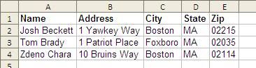
If your data looks like this it is a vertical list:

The VLOOKUP function is, to me, one of the most powerful functions in Excel. In my line of work it is by far the most frequently used formula.

The guts of the VLOOKUP formula has 4 parts. It basically needs to know “what you’re looking up”, “where you’re looking it up”, “the column which contains the data you want to retrieve”, and a qualifier such as “false”.  i.e.=VLOOKUP(what you’re looking up, where you’re looking it up, which column contains the data you want to retrieve, false)

Let’s look at each of these individually.

• What you’re looking up
• This is the piece of data that you want to match in another spreadsheet or dataset. In our example this would be the name.
• This data must match exactly to the other dataset, otherwise the data (birthday) will not be returned.
• Where you’re looking it up
• This is the dataset that contains the data you want to retrieve. It could be on second spreadsheet or a different tab or even on the same tab. In our example this would be the table that contains the birthday.
• You’d select all of the data starting with the column that has the match to step 1 (name) up to and including the column that contains the data you want to retrieve (birthday).
• Which Column contains the data you want to retrieve
• This is probably the trickiest piece of this formula. Since VLOOKUP formulas only work left to right, you need to remember that the data you want to retrieve must always be to the right of your matching data. (In our example, the birthday must be to the right of the name in order for the formula to work properly).
• What we’re looking for here is the column number within the target dataset that contains the data we want to retrieve (birthday). Therefore if the name is in Column A and the birthday is in Column B, you’d strike the “2” key (A=1, B=2). If the name is in Column C and the birthday is in Column E, you’d strike the “3” key (C=1, D=2, E= 3)
• A qualifier
• For simplicity purposes, it’s a good habit to always finish it off with the word “false”. Using the word false in this position tells the formula “Hey, if you don’t find an exact match, don’t give me anything!”
• Without this “false”, it is possible that Excel will return the next closest match. 99 out of 100 times you will not want the closest match, including in our example. I’m sure you don’t want to send Josh Beckett a birthday card on Tom Brady’s birthday, do you? ;o)

So let’s put this to an actual example. Here are the two pieces of data we need:

List with Addresses in a workbook called Addresses.xls

List with Birthdays in a workbook called Birthdays.xls

We want to combine the two so we have one list:

So the VLOOKUP to accomplish looks like this:

 

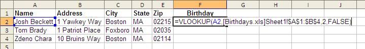
• The first part “What you’re looking up” is the A2. In other words, you want to lookup and match what is in cell A2
• The second part “Where you’re looking it up” is the [Birthdays.xls]Sheet1!$A$1:$B$4. What this tells Excel is that you want to look in the “Birthdays.xls” workbook, on “Sheet 1” in the range of “A1 to B4”. You don’t need to remember the brackets and other symbols as long as you use your mouse cursor to select the data range you need.
• The third part “Which Column contains the data you want to retrieve” is the 2. This tells Excel that the information you want to pull back is in the 2^nd column of the data set you’ve selected (A1 to B4).
• The fourth part, the qualifier, is the word FALSE. As I stated previously, it’s always a good habit to finish the VLOOKUP formula off with the word FALSE.

 

And here is the result:

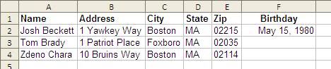
All that’s left to do is to simply copy and paste the formula down to the other rows and your mission is complete.

I tried to make this as simple as possible, but sometimes it is difficult to put into words the actions and requirements of physically doing it. If further clarification is needed, please comment below and I will do my absolute best to help you.