Keeping it in Perspective - The Name Box

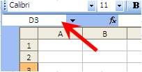
Previously, we spoke about anchoring our data in Excel Formulas by using the dollar sign ($). Well, there is a way of "anchoring" our references without actually using the $ symbol; but we need to name the cell. (We're not technically anchoring the cell, but we'll end up with the same result as if we did anchor it.) Above Column A and to the left of the formula bar is a Name Box that tells us which cell we are in.

We can rename that cell by overwriting that "D3" in that name box to something more meaningful. Using same data as our "Anchor" post, let's say cell D1 contains January Sales and cell D2 contains February Sales. We can easily rename those cells to Jan and Feb respectively. All you have to do is overwrite the D1 with Jan and D2 with Feb.

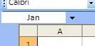
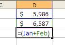
Once that is done, instead of typing in =D1+D2, we can have our formula read =(Jan+Feb).

Other uses

• If you need to get to a particular cell that is buried deep in your data you can access it quickly using the name box. For example, if you know there is a piece of data you need in cell S2806 instead of scrolling across to column S and then scrolling down to row 2806, you can simply type in S2806 in the name box and hit Enter and you will be taken there.

• You can name entire ranges, not just single cells. All you have to do is highlight the entire range THEN name it by typing a meaningful name in the Name Box. Looking back to our VLOOKUP Formula post, if we had named our range of birthdays as "Birthdays" the formula would have looked liked this: =VLOOKUP(A2,[Birthdays.xls]Birthdays,2,FALSE)

This neat little feature can really make Excel life a little easier by being able to quickly and easily trace back formulas!

Keep Excelling!

Do you like this post? Comment below and / or share on Facebook or Twitter!

Going Places? - Hyperlinks

Do you have cells with hyperlinks? Maybe it's an email address or a web address in a cell that you need to change. Editing that cell is not as easy as simply clicking on it! You see, if you simply click on a cell with a hyperlink, it will open that hyperlink! Excel will open you browser and take you to that website, or open up your email client to send an email to that email address!

There are three ways that quickly come to mind to actually select that cell without activating the hyperlink.

The first method I suggest is based on our Using the Name Box blog post. Just type the address of the cell you want to edit in the name box, and Excel will take you there.

The second method I suggest is to simply click the cell beside that one and navigate using your keyboard arrows to the cell that contains the hyperlink.

The third method is using your mouse cursor to click the cell, but don't simply click it - click and hold it for a few seconds. This will bypass the hyperlink activation and allow you to select the cell.

As you can see, Excel is VERY versatile. There is usually more than one way of doing something. Have you found any different way of getting around this? Leave a comment below and let us know!

Keep Excelling!

Do you like this post? Comment below and / or share on Facebook or Twitter!