The Round Formula

Do you need to round your numbers? Maybe get rid of cents in a currency calculation? Do you need to make sure that you don’t end up with half cents? The ROUND function will take care of that for you.

As an example, let’s say you sell fruit. At the end of the day, you sold 25 apples and collected $14.35. This averages out to 57.4¢ each. Obviously there is no such thing as .4 cents! Therefore you would need to ROUND that number. The ROUND formula takes the form of =ROUND(Number or calculation to round, Number of decimal places) Usually, anything dealing with currency or dollars, you will want to round it to 2 decimal places - unless you’re dealing with very large numbers and cents are insignificant; then you’ll want to round to 0 decimal places (dollars only; no cents).

Here’s our example:

And after applying the formula:

Once you are done, you can Copy & Paste Values or simply leave the formula as is. It’s up to you!


NOTE:

If you don’t use the ROUND formula and simply apply the currency formatting, or any other formatting that formats numbers to 2 decimal places; that is only formatting! You only SEE numbers out to 2 decimal places, but the data may still have more. Just keep that in mind when using that type of formatting.


Keep Excelling!

Do you like this post? Comment below and / or share on Facebook or Twitter!

Even or Odd

This is a quick and simple formula that will let you know whether a number is even or odd.

There are instances when you need to know whether a number is even or odd. Let’s say you are calculating sales by sales person. But because the name of your company is “Even Up, Inc” the sales folks get an extra bonus for sales made on even days!

To figure which days are odd and which are even, you can simply use the ISODD or ISEVEN functions.

The result from this formula will be either TRUE or FALSE. If the number is even, you will get TRUE, if it is odd, you will get FALSE. (Obviously, if you use the ISODD formula, you will get TRUE if the number is odd and false if the number is even)

Therefore if you use this in conjunction with the IF STATEMENT formula you can really get your desired result.

Lastly, if you want it to be more dynamic, you can perform your calculations right in this formula by NESTING other formulas or calculations in lieu of the “Bonus!” or “No Bonus” text.



Keep Excelling!

Do you like this post? Comment below and / or share on Facebook or Twitter!

Just In Case – Upper, Lower, & Proper Case Text

Have you ever typed your text in lower case, but changed your mind afterward and would rather have it all in upper case? Maybe you’d rather have the first letter of each word capitalized and wished there was a way that you didn't have to type it all over again? Well there is!!! Without this formula I’m going to tell you about, you would have to start all over and type it all again. Using the nifty UPPER or LOWER or PROPER formulas will take care of it for you. Just select a blank cell (or column) beside the data and type in the formula(s).

The formula for changing everything to upper-case is =UPPER(text or cell to convert)

The formula for changing everything to lower-case is =LOWER(text or cell to convert)

The formula for changing everything to proper-case is =PROPER(text or cell to convert)

It really doesn’t get easier than that!

The next thing you need to do is copy and Paste the Values where you want to display the text (this will most likely be the original cell or column that contained the text in the improper case - unless you want 2 columns with the same data!)

There is one caveat with the PROPER formula: it will capitalize the first letter in any text that follows any character other than a letter. What this means is if you wanted to put “that’s all folks” into proper case, it would result in “That’S All Folks” As you see it capitalized the s after the apostrophe. There is no direct way around this (that I know of) but is not a major issue. Depending on how many I have to change (or how much data I have to look through to find them) what I do is either manually change them one-by-one, or I use a Find & Replace (after I’ve Pasted the Values). I could probably go on, but in the spirit of not confusing  you, I’ll stop right there.

If you have any questions, please post a comment below!

Keep Excelling!

Do you like this post? Comment below and / or share on Facebook or Twitter!

The Paste Special: Values Function

 If you use Excel to create formulas, you will inevitably need to move the data result of those formulas somewhere else. We spoke a little about this in the “Holding Down the Fort – Anchors” post, but in that post what we actually did was move the formula (when we move a formula, as long as its anchored, we move the result also).

But what if you want to move ONLY the data, WITHOUT    the formula? This is where the “Copy & Paste Special - VALUES” comes in to play. By copying the formulas, then selecting the Paste Special option, you can select Values from the dialog box and paste only the result.

Throughout the years and the different versions of Excel, there have been different methods of accessing the Paste Special dialog box. Some have a button the tool bar, while others don’t. Since I don’t know which version you have, there is one method to access the Paste Special dialog box that works with all versions: Alt+E+S. (I find it quicker this way anyway!)

To use this shortcut and go directly to the Past Values function, just add a V to that shortcut: Alt+E+S+V. Striking the Enter Key (or clicking the OK button) will apply your selection (Values) and you will then have removed all the formulas while keeping the values.


Keep Excelling!

Do you like this post? Comment below and / or share on Facebook or Twitter!

Keeping it in Perspective - The Name Box

Previously, we spoke about anchoring our data in Excel Formulas by using the dollar sign ($). Well, there is a way of "anchoring" our references without actually using the $ symbol; but we need to name the cell. (We're not technically anchoring the cell, but we'll end up with the same result as if we did anchor it.) Above Column A and to the left of the formula bar is a Name Box that tells us which cell we are in.

We can rename that cell by overwriting that "D3" in that name box to something more meaningful. Using same data as our "Anchor" post, let's say cell D1 contains January Sales and cell D2 contains February Sales. We can easily rename those cells to Jan and Feb respectively. All you have to do is overwrite the D1 with Jan and D2 with Feb.

Once that is done, instead of typing in =D1+D2, we can have our formula read =(Jan+Feb).

Other uses

• If you need to get to a particular cell that is buried deep in your data you can access it quickly using the name box. For example, if you know there is a piece of data you need in cell S2806 instead of scrolling across to column S and then scrolling down to row 2806, you can simply type in S2806 in the name box and hit Enter and you will be taken there.

• You can name entire ranges, not just single cells. All you have to do is highlight the entire range THEN name it by typing a meaningful name in the Name Box. Looking back to our VLOOKUP Formula post, if we had named our range of birthdays as "Birthdays" the formula would have looked liked this: =VLOOKUP(A2,[Birthdays.xls]Birthdays,2,FALSE)

This neat little feature can really make Excel life a little easier by being able to quickly and easily trace back formulas!

Keep Excelling!

Do you like this post? Comment below and / or share on Facebook or Twitter!

What if ?? – The IF Statement

If it’s Sunny, then I’ll go out; otherwise I’ll stay home. If the Red Sox win, I’ll celebrate, if not, I won’t. These and many others are basic decisions we are faced with on a daily basis. They are so commonplace for us all that we don’t even think of the logic behind our decision making!

Excel offers us a similar function, but this time we will understand the logic. For example, if the month is May, then add up this range of cells, if not add up this other range of cells. If a particular cell is greater than $1000, then display “Good Job!”, otherwise display “Better Luck Next Time”.

The most basic explanation of the IF statement is this: IF(Something, This, That). The key is to remember that the commas are your deciders. Mentally replace the first comma with “THEN” and the second comma with “OTHERWISE”. So verbally, the logic would sound like IF(Something THEN This OTHERWISE That). Armed with this knowledge, anyone can write an IF Statement in Excel quickly and easily. (Some folks use the terminology IF, THEN, ELSE; either way it means the same thing.)

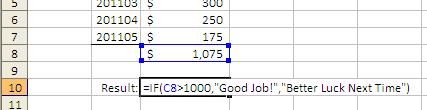
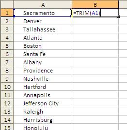
Here is a visual representation of the last example.

The formula first checks whether or not the cell has a value that is greater than $1000. If the argument is positive (in other words the answer is yes - it does have a value over $1000), it will display the words “Good Job!”, if the argument is negative (in other words the answer is no - it doesn’t have a value greater than $1000), it will display “Better Luck Next Time”.

Multiple IF’s

You can also nest IF Statements. For example: If it’s Sunny, and if the Red Sox are playing, then I’ll go to the game; otherwise I’ll stay home. A formula with those arguments would look like: =IF(Sunny, IF(Red Sox Playing, Go to the Game, Stay Home),Stay Home)

As you see, the second IF Statement sits completely between the “THEN” comma and the “OTHERWISE” comma (including the closing parentheses). This means that if, and only if, the first IF statement (Is it Sunny?) results in a positive result (Yes, it's Sunny), it will look at this second IF Statement. If the result of the first IF Statement is negative (It's not Sunny), it will bypass the second IF Statement completely and go straight to "Stay Home".

Depending on your version of Excel, you may only be able to nest up to 7 IF Statements in one cell.

Tell me what you think of my explanation of the IF Statement by posting a comment below!

Keep Excelling!

Do you like this post? Comment below and / or share on Facebook or Twitter!

It’s in there! – Nesting

Nesting is not a formula or function. What it means in Excel is that you can include a formula within a formula. You are “nesting” a formula within a different formula. The best way to explain this is to give you a visual representation. We’ll look at nesting a TRIM function  within a VLOOKUP formula, but remember that there are many formulas that can be nested within each other (I have nested VLOOKUP formulas within other VLOOKUP formulas!) Generally, if you need to perform a separate function to get what you need for a different formula, it can be nested.

Let’s say we have a list of State Capitals (just as we did for our TRIM function post) and we want to find each capital’s state.

If you simply created the VLOOKUP with the data as is (with extra spaces) it would look like this and you would get an #N/A error: =VLOOKUP(A1,$D$1:$E$16,2,FALSE).

So what you want to do is add in the TRIM function within that formula. As you see from our original TRIM blog-post, the formula is =TRIM(A1). Therefore by “nesting” the two the VLOOKUP would now look like this: =VLOOKUP(TRIM(A1),$D$1:$E$16,2,FALSE).

 

If you remember, the first part of the VLOOKUP formula is “What you’re looking up”. In this case, we’re looking up the result of TRIM(A1) formula. I hope this makes sense... If you need further clarification, please post a comment below.

Keep Excelling!


Do you like this post? Comment below and / or share on Facebook or Twitter!

Going Places? - Hyperlinks

Do you have cells with hyperlinks? Maybe it's an email address or a web address in a cell that you need to change. Editing that cell is not as easy as simply clicking on it! You see, if you simply click on a cell with a hyperlink, it will open that hyperlink! Excel will open you browser and take you to that website, or open up your email client to send an email to that email address!

There are three ways that quickly come to mind to actually select that cell without activating the hyperlink.

The first method I suggest is based on our Using the Name Box blog post. Just type the address of the cell you want to edit in the name box, and Excel will take you there.

The second method I suggest is to simply click the cell beside that one and navigate using your keyboard arrows to the cell that contains the hyperlink.

The third method is using your mouse cursor to click the cell, but don't simply click it - click and hold it for a few seconds. This will bypass the hyperlink activation and allow you to select the cell.

As you can see, Excel is VERY versatile. There is usually more than one way of doing something. Have you found any different way of getting around this? Leave a comment below and let us know!

Keep Excelling!

Do you like this post? Comment below and / or share on Facebook or Twitter!

Holding Down the Fort - Anchors

After you create a formula, you may not simply be able to paste the results in a different area such as a new worksheet or a different workbook. If the formula arguments are still in the cell you're trying to copy over to a new cell, what you're doing is actually copying over the formula!


When creating a formula, Excel doesn't look at the data in the cell, and it doesn't necessarily look at the address of the cell (A2, B5, D12, etc) either. It looks at the relative position of a cell in reference to the cell that in which the formula is being created. For example, if you're putting a formula in cell D3 that is adding cells D1 & D2, you would type =(D1+D2). What Excel is understanding by that is add "me minus two rows" + "me minus one row". Therefore, if you were to copy that formula and past it to cell F37, it would read =(F35+F36) which is, in reference,  "me minus two rows" + "me minus one row".

In order to be able to copy that formula to cell F37 or any other cell without changing the reference (D1+D2) you need to "Anchor" the cell references. This is done by adding a dollar sign ($) to either or both of the cell references, row and column. By adding an anchor to the column reference, the column is anchored ($D1+$D2), and by adding an anchor to the row reference, the row becomes anchored (D$1+D$2). By adding the anchor to both the column and row references, they both become anchored ($D$1+$D$2).

As you're typing in the formula, you can add anchors by simply striking the "F4' key before the next part of the formula (comma, parentheses, plus sign, etc). This allows you to cycle through the anchors: pressing the F4 key once will anchor both the row and column, pressing it again will only anchor the row, one more time and it will anchor the column, pressing it a fourth time will remove all anchors and basically anchor none (pressing it one more time will start the cycle over again).

So the next time you copy your formulas over to a new cell and you get an error (#N/A, #VALUE!, etc) it's probably because your references are not anchored. A quick fix will take care of it for you.


Keep Excelling!

Do you like this post? Comment below and / or share on Facebook or Twitter!

Lose the Excess – TRIM Function

Are you trying to perform a VLOOKUP Formula but it’s not working? Even though you KNOW the formula is right AND you KNOW the data is there? The issue MAY just be that there are leading or trailing spaces that you don’t see. After all, in an Excel cell the words “Boston” and “Boston     ” LOOK identical, but they’re not (go ahead and try it, we’ll wait for you to come back!)

As I stated, they are not identical, and thus the formula will not find a match and return a “#N/A” error.

Getting rid of these spaces is as simple as typing in

 =TRIM(cell that contains extra spaces)

 

After removing the extra spaces, you may or may not see a difference; depending on where the spaces – leading spaces (before your data) or trailing spaces (after your data). Either way, this MAY be all that is needed to make your formula work.

Keep Excelling! 

Do you like this post? Comment below and / or share on Facebook or Twitter!

Auto Column Width

If you routinely have data that fills up a cell and then some, Excel offers a quick and easy way to see it all.

As you may know, you can easily place your cursor on the line to the right of the column header you’d like to adjust, click and drag to your desired width.

This may be all you need if the data that is visible on the screen is all you have, but what about the data that is down on row #2437? It could be wider still!

My quick and easy way is just a variation of the “click and drag” method and adjusts the column width of all the data in that column. Instead of clicking and dragging the column which you want to adjust, simply double-click the same line. (Just as we adjusted the Row Height yesterday, we can also adjust multiple columns at the same time. Just follow the same instructions of selecting multiple rows, but apply it to columns instead)

As you can see, the column adjusted itself to the width of the largest cell in that column; in this case “September”

Keep Excelling!

Do you like this post? Comment below and / or share on Facebook or Twitter!

Auto Row Height

On the rare occasion that a particular font size is bigger than the height of cell, you may need to adjust the height of the rows on the Excel sheet so you can see all the data easily. You can adjust each row one at a time; however if you have many rows that need adjusting, it is much quicker to adjust them all at the same time.

The first ting you need to do is select all the rows that need to be adjusted. Using your mouse, position your cursor on the row header (numbers down the left side of the Excel sheet), then click and drag from the first row that contains data down to the last row that contains data. (If you have a lot of data, you may want to press Ctrl-a; this will select the entire Excel worksheet)

 

Now position your mouse cursor between any two of the selected row headers and double-click.

 

As you can see, all of the rows have adjusted to the proper height.

That’s all for today, come back tomorrow and we’ll talk about adjusting the Column Width.

Keep Excelling!!!

Do you like this post? Comment below and / or share on Facebook or Twitter!

How Long Is It? - LEN

If you need to know the number of characters in a cell, Excel can make the task of counting every letter, space, number, or other character MUCH simpler. But why would you need to know how many characters you have in a cell? I’m sure there are a plethora of reasons. For me, as a sales analyst, I occasionally need to work with zip codes.

Zip codes in the northeastern US all start with the number 0 (the zip code for Fenway Park in Boston is 02215, while one of the zip codes for Hartford CT is 06105) If the column that contains the zip codes is not formatted as text, then the zip codes that start with a zero have the leading zero removed. Excel thinks it’s a number (doesn’t know it’s a zip code) and therefore, 02215 as a number translates to 2215 which is what Excel displays. But if you try to mail a letter to zip code 2215, it will be returned faster than a Jonathan Papelbon high-fastball!

Therefore, in order to find which zip codes are in error (only 4 characters long as opposed to the regular zip codes that have 5 characters), the easiest way is to use the LEN formula. The LEN formula counts all characters including spaces within a cell.

As with many Excel formulas, the formula is simple once you know it exists! All you have to do is type =LEN(cell). That’s it! (You count the length of any piece of info, not just what's in a cell; just put the data you want to count in between the parenthesis.)

By using this formula in the zip code context I mentioned, you can easily see which zip codes are in error. By applying this to all zip codes on a worksheet, you can then sort them all and using the CONCATENATE formula you can correct them all quickly and easily.

And the result that you can easily copy and paste back to the original column that contains the zip codes:

Keep Excelling!

Do you like this post? Comment below and / or share on Facebook or Twitter!

Putting It All Together - Concatenate or &

Sometimes the data we need may be in separate columns. Excel offers a very simple way of bringing it all together.

Consider this post a prequel to the post for the FIND function (http://excelblast.blogspot.com/2011/04/find-function.html), because our result here is our beginning data there.

We have a list of US Presidents and their first and last names are in separate cells. Using the CONCATENATE formula, you can quickly and easily bring them together into the same cell. The formula, takes the form of =CONCATENATE(something, something else, one other thing). You can concatenate up to 30 “things”.

Here’s an example:

As you see, we’ve concatenated the President’s first name, a space, and their last name.

Now, not to confuse you, but if you find it hard spelling concatenate, you can simply use the ampersand (& - and no you don’t have to spell that one either!)

As you can see, we've combined the same components however, instead of using the word CONCATENATE and commas in the formula, we simply use the ampersand (&) between the components.

And the result:

Keep Excelling!!!


Do you like this post? Comment below and / or share on Facebook or Twitter!

LEFT, MID, & RIGHT

Have you ever had the need for data that's in a cell, but not the entire cell? When the need arises to dissect a cell, Excel has you covered.

Whether the data you need is in the beginning of a cell, the middle of a cell, or the end of a cell - there's a formula for that.

Where I work, we use a lot of dates in the format of YYYYMMDD (today is 20110430). Let's say you want to separate those into separate cells so you can subtotal them by their particular month. You need to figure out a way to split the cell so you can have the data you need. Because all of the data in this example is 8 characters long, there are a couple of different ways you can accomplish this; but today we're going to focus on using the LEFT, MID, & RIGHT formulas. Let's get right to it.

LEFT

In order to extract the year from from the data, you use the LEFT formula. Before using this formula, you need to know two things; the cell that contains the data and the length of the data you'd like to extract. The formula takes the form of =LEFT(Cell that contains the data, the number of characters you'd like to extract). Here's a visual example:

And the result:

MID

To extract the month it's a little trickier (because it's in the MIDdle of the data), but it's still just as easy. This time you need to know THREE things before you can use the formula; the cell that contains the data, the position of the first character you want to extract, and the length of the data you'd like to extract. The formula takes the form of =MID(Cell that contains the data, the position of the first character you want to extract, the number of characters you'd like to extract). Here's a visual example:

And the result:

RIGHT

Using the RIGHT formula is just like using the LEFT formula except you're starting from the right instead of the left (it it weren't obvious enough!) Therefore, you need to know the same two things; the cell that contains the data and the length of the data you'd like to extract. The formula takes the form of =RIGHT(Cell that contains the data, the number of characters you'd like to extract). Here's a visual example:

And the result:

Here is the final result:

I hope I've explained it easy enough! At a later date, I'll explain the other method we could have used to accomplish this task - Text to Columns. As I stated earlier, only because every cell has the same amount of characters AND they are all in the same position (the first four positions are the year, the next two are the month, and the last two are the day) could we use this different method.


Until next time... Keep Excelling!!!

The FIND Function

If you need to know in which position a particular character is in a cell, the FIND function is exactly what you need.


Let's say you have a list of names. Both first and last name in one cell separated by a space. If by chance you want to know in which position the space is in, the formula is as simple as =FIND("What you're looking for", The cell that contains what you're looking for). That's it!


Here's a visual example.

Just remember that if what you're looking for is text, you need to enclose the search item in quotes (to find a space, we use " ")

As you can see the result is 7, meaning the space is the 7th character within that cell.

One other thing to keep in mind is that the formula will only find the first instance of what it is looking for. As you see in the example above on row 6, "John Quincy Adams" has 2 spaces, however the result of the formula is 5, meaning the space is in the 5th position. Once ANY formula finds what it is looking for, it stops looking and thus there is no mention of the 2nd space. (There is a way to find the 2nd and subsequent spaces, that's a little more advanced so it will be another topic for a later date).
 

Working with Multiple Tabs

Do you ever work with an Excel workbook that has multiple worksheets (tabs)? If you do, you may want to take note of this quick shortcut.

If you’re using your mouse to click on things within the worksheet, then it may make sense to simply use the mouse to click on the desired tab. However, if you’re like me, your hands are on the keyboard most of the time.  Therefore to navigate between tabs, whether its for formulas or simply comparing data (there’s a formula for that!) it is MUCH easier and quicker to simply press the “Ctrl - Page Up” or “Ctrl - Page Down”.

If you would like to navigate one tab to the left, you press “Ctrl - Page Up”. If you would like to navigate one tab to the right, you press “Ctrl - Page Down”. It really can’t be simpler!

Do you find this useful? Post a comment below and let me know what you think!

The VLOOKUP Formula

Do you have or have you had a dataset that had some data, but wasn’t complete? Maybe you have a list with your family & friends addresses. On another list, maybe you have a list with everyone’s birthday. If you wanted to consolidate both of these lists into one, how would you get the birthdays into the other list or vice-versa? You could manually type them all in, but that could take quite a bit of time depending on how large your list is.

In Excel, we have a formula called VLOOKUP. VLOOKUP stands for vertical lookup. You can take a piece of data/information and look it up into a vertical list (stay with me) and retrieve another piece of data/information.

If your data looks like this it is a vertical list:

The VLOOKUP function is, to me, one of the most powerful functions in Excel. In my line of work it is by far the most frequently used formula.

The guts of the VLOOKUP formula has 4 parts. It basically needs to know “what you’re looking up”, “where you’re looking it up”, “the column which contains the data you want to retrieve”, and a qualifier such as “false”.  i.e.=VLOOKUP(what you’re looking up, where you’re looking it up, which column contains the data you want to retrieve, false)

Let’s look at each of these individually.

• What you’re looking up
• This is the piece of data that you want to match in another spreadsheet or dataset. In our example this would be the name.
• This data must match exactly to the other dataset, otherwise the data (birthday) will not be returned.
• Where you’re looking it up
• This is the dataset that contains the data you want to retrieve. It could be on second spreadsheet or a different tab or even on the same tab. In our example this would be the table that contains the birthday.
• You’d select all of the data starting with the column that has the match to step 1 (name) up to and including the column that contains the data you want to retrieve (birthday).
• Which Column contains the data you want to retrieve
• This is probably the trickiest piece of this formula. Since VLOOKUP formulas only work left to right, you need to remember that the data you want to retrieve must always be to the right of your matching data. (In our example, the birthday must be to the right of the name in order for the formula to work properly).
• What we’re looking for here is the column number within the target dataset that contains the data we want to retrieve (birthday). Therefore if the name is in Column A and the birthday is in Column B, you’d strike the “2” key (A=1, B=2). If the name is in Column C and the birthday is in Column E, you’d strike the “3” key (C=1, D=2, E= 3)
• A qualifier
• For simplicity purposes, it’s a good habit to always finish it off with the word “false”. Using the word false in this position tells the formula “Hey, if you don’t find an exact match, don’t give me anything!”
• Without this “false”, it is possible that Excel will return the next closest match. 99 out of 100 times you will not want the closest match, including in our example. I’m sure you don’t want to send Josh Beckett a birthday card on Tom Brady’s birthday, do you? ;o)

So let’s put this to an actual example. Here are the two pieces of data we need:

List with Addresses in a workbook called Addresses.xls

List with Birthdays in a workbook called Birthdays.xls

We want to combine the two so we have one list:

So the VLOOKUP to accomplish looks like this:

 

• The first part “What you’re looking up” is the A2. In other words, you want to lookup and match what is in cell A2
• The second part “Where you’re looking it up” is the [Birthdays.xls]Sheet1!$A$1:$B$4. What this tells Excel is that you want to look in the “Birthdays.xls” workbook, on “Sheet 1” in the range of “A1 to B4”. You don’t need to remember the brackets and other symbols as long as you use your mouse cursor to select the data range you need.
• The third part “Which Column contains the data you want to retrieve” is the 2. This tells Excel that the information you want to pull back is in the 2^nd column of the data set you’ve selected (A1 to B4).
• The fourth part, the qualifier, is the word FALSE. As I stated previously, it’s always a good habit to finish the VLOOKUP formula off with the word FALSE.

 

And here is the result:

All that’s left to do is to simply copy and paste the formula down to the other rows and your mission is complete.

I tried to make this as simple as possible, but sometimes it is difficult to put into words the actions and requirements of physically doing it. If further clarification is needed, please comment below and I will do my absolute best to help you.

Find & Replace

One thing you'll find out about me is that I am a HUGE fan of shortcuts. If there is a faster way of doing something and will get me the exact same results, I'm all over it!

Today's topic is about Excel's "Find" & "Find and Replace" functions.

There are many ways to do this, but I'm going to touch upon the methods I use (this is my blog after all :o)

Reaching up for my mouse to click on something to find something simply takes too long for my liking.  therefore, while I already have my hands on my keyboard, i simply press "Ctrl f" for the "Find" dialog box and "Ctrl h" for the "Find and Replace" dialog box.

Enjoy!

My Favorite Excel Function

OK, let’s get down to some Excel business. This post will focus on my absolute favorite Excel shortcut. You'd think that for someone like me who uses Excel extensively day in and day out it'd be something extravagant; NOPE! My favorite Excel function is simply "Ctrl-z"; the "undo" function! If I had a nickel for every time this nifty little function has saved my behind, I'd be a rich man! 

Sure you can easily grab your mouse and click on the "Undo Arrow" or even click on Edit / Undo

A Little About Me.. & the Blog...

A little bit about me...

You may be asking who are you and why do you have an Excel blog. I have to say that's a great question. I've been asking myself who I was for MANY years. And I've also been asking myself why I DON'T have an Excel blog for years!

Well, my name is Ray and I've been an Excel addict for over 10 years, ever since I was thrown into a job where I needed to use it! You see, I had been a truck driver for years but I had always had a love for computers.

First Post!

This is my first post here on my new blog!

(applause)

Thank you, thank you, thank you!!! You're too kind!!!